04. Execute the program
1. Prepare Data for MCMC:
Before running the MCMC, all data and input files must be properly prepared and placed in the correct directories. The data files (e.g., *.ph, *.hv, *.rf) should be stored in {Project}/data/{sta}_data.
The input files, including the model file
(mod.{sta}),
the parameter control file
(in.para_{sta}),
the data control file
(in.data_{sta}),
and the connector file
(in.connector),
will be automatically generated and placed in the same directory after running
01_prepare_data.sh.
> Before running, open the script
01_prepare_data.sh
and update the
{Project}
name to match the current project.
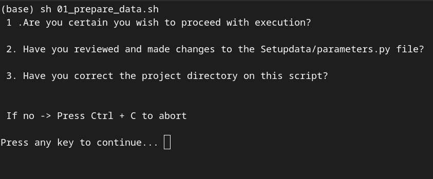
Figure 4.1: execute the
01_prepare_data.sh
to set up the input files.
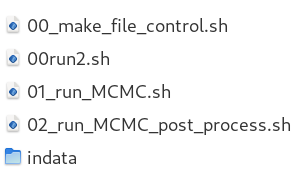
> Check other important files. Make sure that those file stay in {Project}/MonterCarlo
|
|
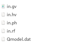
Figure 4.2: (Left) Files placed in {Project}/MonterCarlo to control the run, and (Right) template files in {Project}/MonterCarlo/indata used when input data are not fully available.
> If everything works correctly, the data files and the four input files should be located in {Project}/data/{sta}_data
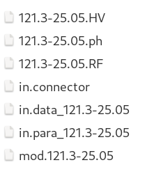
Figure 4.3: Files placed in
{Project}/data/{sta}_data
after running the data preparation script. Note that 121.3-25.05 here is the station name.
2. Execute the MCMC:
> Open the
02_do_MCMC.sh
change the project name.
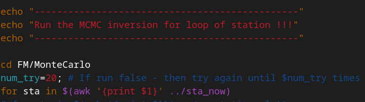
Figure 4.4: Location of
{Project}
name in script
02_do_MCMC.sh
. The number of try if fail also marked nearby as
num_try
> The current script is set to retry the run up to 20 times if it fails (num_try)
> If you change anything on the code, choose YES to recompile the program
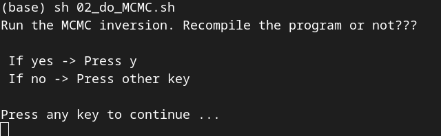
Figure 4.5: Script screen output during execution
sh 02_do_MCMC.sh.
After executing the script, the file {sta}.control will be generated in {Project}/data/{sta}_data/. This file can also be used to check all input filenames and connector values.
3. How the MCMC works
The code mainly runs in two main steps + 1 plot step:
(1) Run MCMC sampling: The code performs MCMC sampling
by drawing model parameters, generating posterior samples, and calculating
the misfit between synthetic and observed data. Models that satisfy the
acceptance condition are stored in binary files.
This step is executed by sh 02_do_MCMC.sh, which calls the sub-script
{Project}/MonterCarlo/01.run_MCMC.sh.
(2) Post-process posterior models: The code reads the binary
files from step (1) and selects a subset of models based on the settings
in {Project}/data/{sta}_data/in.connector. It then calculates the
average model, standard deviation, and performs forward modeling to
generate synthetic data for plotting.
This step is executed by sh 02_do_MCMC.sh, which calls
{Project}/MonterCarlo/02.run_MCMC_post_process.sh.
(3) Plot results: The final figures are generated using the
selected models and corresponding synthetic data from step (2). This
step is excuted by AnalyzeResult/inversion_plot_vfinal_flex.py.Output figures are saved in {Project}/MonterCarlo/{sta}/*.png.
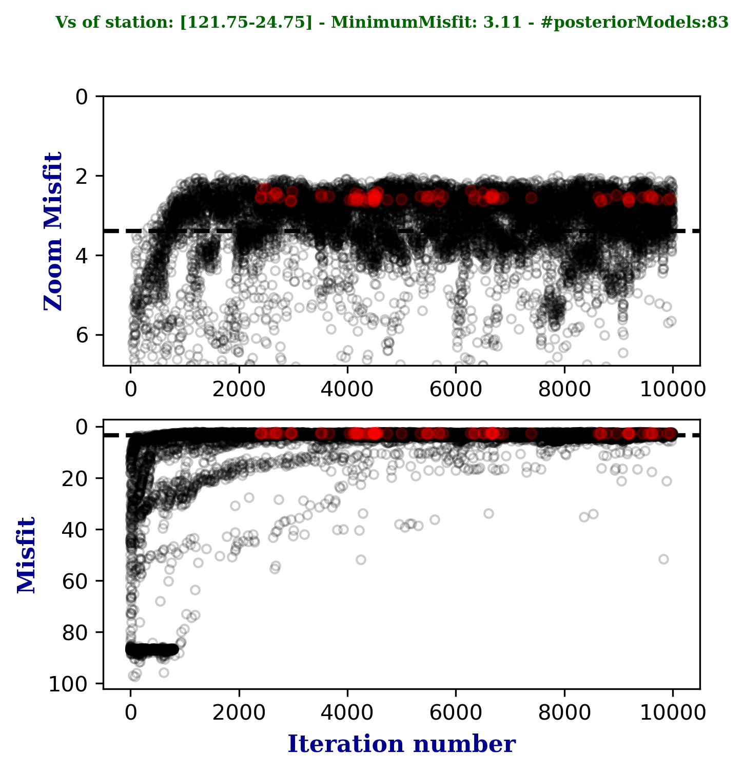
Figure 4.6: Example of output figure {sta}_IterVsMisfit.png. showing the posterior-selected models (red) over the full set of posterior models (gray).

Figure 4.7: Example of output figure {sta}_MCMC.png. showing the final results, posterior distribution, minimum-misfit model, initial synthetic model, and data from the input model. Observed data are plotted as black circles. Note that: the plotstyle here set as gradient style for the 1D posterior model.