01. Prepare input files
-
Before running the MCMC inversion, the first step is to prepare all
input data and input 1D model in a clear and consistent format. Think of
this step as setting up everything the inversion needs to “learn” the
Earth structure.
1. Phase velocity (Vph): Directly constrains the absolute velocity structure of the model. It is one of the most important datasets for defining the overall velocity with depth.
2. Group velocity (Gv): Provides additional constraints on the velocity structure, particularly useful for improving resolution at different depth ranges depending on the period sensitivity.
3. Rayleigh-wave ellipticity (HV): Provides relative constraints on the velocity structure. Since HV is the ratio of radial to vertical motion, it is sensitive to impedance contrasts and shallow structure but does not directly constrain absolute velocity values.
4. Receiver Functions (RF): Provide relative constraints on the velocity structure. RFs are referenced to the P-wave arrival and are highly sensitive to discontinuities (e.g., layer boundaries), but they do not directly constrain absolute velocities.
All input datasets must be stored in the directory: {Project}/data/{sta}_data/ , with filenames following the convention {sta}.*.
Each data type is identified by a specific file extension:
.ph for phase velocity (Vph)
.gv for group velocity (Gv)
.hv for Rayleigh-wave ellipticity (HV)
.rf for receiver functions (RF)
-
This consistent naming and directory structure allows the inversion code
to automatically locate and read the required input files for each
station. **Note: you no need to have all types of data to run the
inversion.** The code can work well with single type of data (e.g., only
Vph or only RF), however, using multiple datasets will help better
constrain the model and improve the reliability of the result.
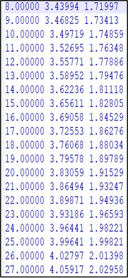
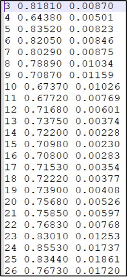
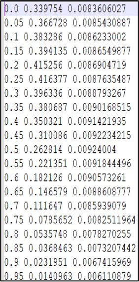
Input file format:: Each input data file is stored in plain text format with no header. The data are arranged in 3 columns, representing:
-
Column 1: Period
-
Column 2: Observed value (e.g., Vph, Gv, HV, or RF amplitude)
-
Column 3: Uncertainty (e.g. Standard deviation)
All values should be in float format and separated by whitespace. Each row corresponds to one measurement point.
|
|
|
| (a) | (b) | (c) |
Figure 1.1: Example of input data file (3-comlumns) of Vph (a) – HV (b) – RF (c).
Notes for Berg: (see Supplementary material for more details)
A) You may need to scale the amplitude of provided receiver functions.
Here I am using a Gaussian width of 3.0 and a ray parameter of 0.06, but I scale the amplitudes of the receiver functions as:
JointInversionRF_input = RFamp / 1.7
Scaling information from (final table):
http://eqseis.geosc.psu.edu/cammon/HTML/RftnDocs/seq01.html
B) Be sure to include 0.00 s time.
I linearly interpolate back to estimate this point if it is not provided.
C) All receiver functions should have the same sampling rate.
The memory allocation size is currently set up for a 0.05 s sampling rate from 0 to 10 s. The RF data allowance in the joint inversion is set as:
- maxdata = 1024 in Codes/MCMC_flex/RF/rfi_param.inc. Note that this should be a power of 2, i.e., 2X, where X is a positive integer.
If you have more data points (a higher sampling rate or a longer receiver function), you may need to increase this value.
D) Check that the receiver functions are set correctly in Codes/MCMC_flex/CALforward.C:- Gaussian width (
float gau = 2.5) - Ray parameter (
float slow = 0.06)
-
II. Input 1D velocity model: The input reference model is used as
the starting velocity model for the inversion. Based on this model, the
code performs forward modeling to generate initial synthetic data (e.g.,
Vph, HV, RF). The 1D model must be placed in:
**{Project}/Vel_mod/{model_name}** as
depth – Vs – Vp. All values should
be in float format and ordered consistently with depth.
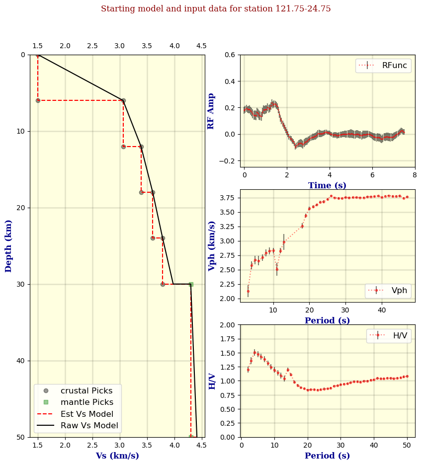
Figure 1.2: Example of the 1D model and input data after running
01_prepare_data.sh.