02. Control files

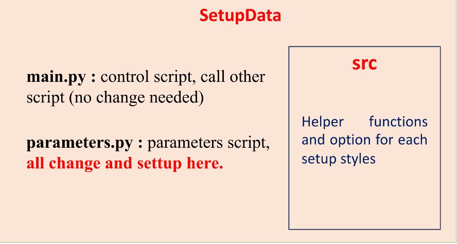
During this step, model parameterization is defined based on the input 1D velocity model and is automatically handled by the scripts in the SetupData folder. You still need to manually define some key parameters. The script will read the input model and convert it into the parameterized form required for the MCMC inversion.

The script also prepares and links all necessary files, including the model file (mod.{sta}), parameter file (in.para_{sta}), data likelihood file (in.data_{sta}), and connector file (in.connector). This ensures that the inversion code can correctly read and use all required inputs. This step is important because it defines the model space that the MCMC algorithm will explore. All parameters can be mainly set in the (SetupData/parameter.py) file.

1. Convert 1D model to mod.{sta}:

To convert the 1D model into the input required for the MCMC workflow, several parameters need to be considered, including:

• Mod_type_flag: choose the model input style. If = 1, use gradient style; if = 2, use B-spline style to smooth the model.

• Vel_mod_uniform_flag: choose whether to use one model for all stations or assign a separate model for each station. If = 1, use model name define later in ({mod_file}) for all; if = 0, use all model in Vel_mod direcotory under {mod_file}/{sta} .

• sed_flag, man_flag: setup the model with sedimentary layers and/or mantle layers (0 for no, 1 for yes).

• sed_value: when **sed_flag** = 1, use **sed_value** to define the initial values of the sedimentary layer in the input model.

• sednpara, crustnpara, mantlenpara: when **mod_type_flag = 2** , these parameters are active and used to define the number of control points for each group of layers.

• sublay_thickchange: control parameter for sublayers variation (mainly focus on crustal group).

Other parameters also need to be taken into consideration (scroll-down to find them):

• dds, ddc, ddm: define the sub-layer thicknesses for the sedimentary, crustal, and mantle groups. Regardless of how many sub-layers are defined in the input 1D model, these parameters control how the model is parameterized during inversion. Note that the current setting supports a maximum of 100 sub-layers across all three groups combined.

→ After running the script 01_prepare_data.sh, the model for each station will be generated in {project}/data/{sta}_data/mod.{sta} with the proper value structure.

Example of input model in bspline style:

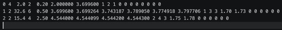
Figure 2.1: The input model setup in B-spline style.

Column 1: layer ids (0,1,2,…: important used on the code)

Column 2: model parametrization type flag (4: linear; 2: cubic B-splines; 1: Layerized)

Column 3: layers thickness (in km)

Column 4: Number (N) of values that describe the layers (linear: number of points, b-spline: number of control points, layered: number of layers)

Column 5: (modified): the values of dds, ddc, ddm for each group layer.

Column 6 to 6 + N: velocity values/controls velocity values at each points

• If layered model setting: if column 2 = 1 (layered), N values will be added after the first 6 + N parameters to represent the sub-layer thickness ratios relative to the total thickness of the group. For example, in group index 1 with group layer = **32.6** km, if the value at position *(6 + N + 1)* is **0.1**, then the thickness of that sub-layer is: total group thickness × ratio = **32.6 × 0.1 = 3.26 km**.

• New version update: If Vpflag = 5, N additional values will be added after 6 + N (for layered) + N parameters to represent the Vp/Vs values of each group. These values are considered as the base values (at 0% perturbation).

Column [size - 11]: define the Rflag, 1 (Brocher’s 2005 paper); 2 (Perturbation relative to reference velocity – Kaban, M. K et al. (2003), Density of the continental roots [use for mantle]); 3 (1.05, for water).

Column [size - 10]: define the Qflag, 0 (input), 1 (water: 0/57882); 2 (sediment,160/80); 3 (crust,600/1368), 4 (mantle,417/1008)

Column [size - 9]: set Vpflag, (see CALgroup.C get_Vp) calculate the coresponding Vp-model from input 1D model: 1 (Brocher, 2005); 2: (AK135, 120km, vpvs=1.789); 3 vpvs = vpvs \[where vpvs is set at Column [size-8] and vpvs1 is set at Column [size-7]]; 4 use relationship vp = vs\*(1.373+2.022/vs)

Column [size-8 & size-7]: vpvs and vpvs1 values used by Column [size-9] if Column [size-9] = 3

Other columns: current unset.

New version update:

Figure 2.2: Example of the input model configured in gradient style. Note that this example does not include sedimentary layer settings. In row 1, 4 velocity values are assigned in columns 6 to 9, while 4 thickness-ratio values are assigned in columns 10 to 13. Another 4 values are added afterward to represent the background Vp/Vs values for each sublayer.

2. parameter file: in.para_{sta}

This file is used to control which parameters are perturbed, the perturbation style, the perturbation range of each parameter, and the step size for each parameter perturbation. All the parameter can modify in the script SetupData/parameter.py

New version update: add the part for Vp/Vs perturbation.

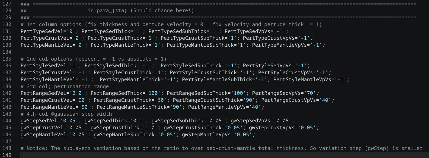
Figure 2.3: Example of parameter control settings for generating in.para_{sta}.

The parameters are organized line by line according to the number of parameters. The current setup generates the parameter file with a number of velocity/crustal thickness perturbations consistent with the number of values in mod.{sta} + number of group thickness change (e.g. sediment thickness and crustal thickness).

New version update: add the part for Vp/Vs perturbation.

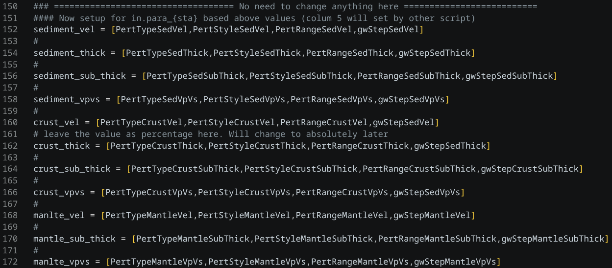
Figure 2.4: Values arrange to velocity and thickness write into in.para_{sta}.

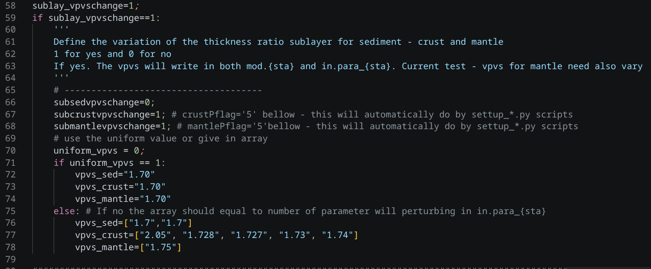
Figure 2.4.1: Values of Vp/Vs arrange to write into in.para_{sta}.

The parameter values are arranged following the logic below:

Column Information:

Column 1: perturbation type flag: (0 = values to be perturbed), (1 = thickness to be perturbed)

Column 2: perturbation style flag: (1 = absolute perturbation), -1 = relative perturbation (in %)

Column 3: perturbation range

Column 4: gaussian step width

Column 5: group layer id (consitent with group id in mod.{sta} file)

Column 6: sublayer id (consistent with number of value each group in mod.{sta} file)

Note: All the ids count from 0

Row Information:

Rows group 0: (if sediment layers are set) : Sediment layer Vs perturbation range (min and max range of velocity)

Rows group 1: Crustal layer Vs perturbation range (min and max range of velocity/bspline)

Rows group 2: (if mantle layers are set) : Manle layer Vs perturbation range (min and max range of velocity/bspline)

Rows group 3: (if sediment layers are set) : total sediment thickness pertubation

Rows group 4: (if crusl and mantle layers are set): total crustal thickness pertubation

Rows group 5: (if set) : Sediment layer thickness perturbation range (top & bottom thickness range of sublayers)

Rows group 6: Crustal layer Vs perturbation range (top & bottom thickness range of sublayers)

Rows group 7: (if set) : Manle layer Vs perturbation range (top & bottom thickness range of sublayers)

• New version update:
Rows group 11-15: If Vpflag = 5, 5 rows for Vp/Vs perturbation will be added to the parameter file. These Vp/Vs perturbations are referred to the corresponding velocity parameters (Vs) and are used to calculate the Vp model.

New version update: add the part for Vp/Vs perturbation.

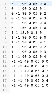
Figure 2.5: Example of values in in.para_{sta} for the case with only crustal and mantle groups in a 1D model. The first 6 rows correspond to velocity perturbations defined in mod.{sta} (5 crustal layers and 1 mantle layer). Row 7 represents the total crustal perturbation, the next 5 rows represent sublayer thickness variations, and another 6 rows (from 13 to 18) are added afterward for Vp/Vs perturbations corresponding to each velocity parameter.

Some important notes:

n1. The number of velocity perturbation group consistent with the number of values in input model {Project}/data/{sta}_data/mod.{sta}. We can check the number of velocity perturbation for each group equal the number in column 4 of input model.
n2. The crustal thickness can vary only when mantle group is set.
n3. The mantle thickness perturbation is not necessary (normally it is the last group layer or not set). If the crustal thickness varies, the mantle thickness will also vary accordingly to keep the total thickness unchanged.
n4. Sub-layer variation rows: these rows are only created when the model is in layered style (= 1 in column 2 of {Project}/data/{sta}_data/mod.{sta}).

⇒ After running the script 01_prepare_data.sh, the model for each station will be generated in {project}/data/{sta}_data/in.para_{sta} with proper value structure.

3. data file: in.data_{sta}
This file is used to control which data are used and the weight assigned to each data type in the likelihood misfit function. All parameters can be modified in the script SetupData/parameter.py

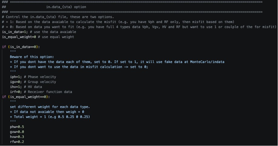
Figure 2.6: Parameters defined in Setupdata/parameters.py that are transferred to {Project}/data/{sta}_data/in.data_{sta}.

is_in_data: flag to use the data that exist in the {Project}/data/{sta}_data directory. If set 0 = not check the avaiable data; if set 1 check the avaiable data.

• if is_in_data = 0: and a data type is set as available (e.g., iph = 1) but the corresponding file ({sta}.ph) does not exist in iph = 1 but the corresponding file data/{sta}_data, then the program will use a temporary file from {Project}/MonterCarlo/indata/* instead.

is_equal_weight: flag for equal (1) or non-equal (0) likelihood weighting.

The parameter values are arranged following the logic below:

Rows Information:

Row 1: data exist for Vph (0 = no, 1 = yes) – auto check file exist on {Project}/data/{sta}_data/{sta}.ph or use iph above if is_in_data = 0.

Row 2: data exist for Gv (00 = no, 1 = yes) – auto check file exist on {Project}/data/{sta}_data/{sta}.gv or use igv above if is_in_data = 0.

Row 3: data exist for HV (0 = no, 1 = yes) – auto check file exist on {Project}/data/{sta}_data/{sta}.HV or use ihv above if is_in_data = 0.

Row 4: data exist for RF (0 = no, 1 = yes) – auto check file exist on {Project}/data/{sta}_data/{sta}.RF or use irf above if is_in_data = 0.

Row 5: flag for likelihood weighting (is_equal_weight).

• If set to 1, the weight is equally distributed among all available data types (e.g., 2 types → 0.5 / 0.5; 3 types → ~0.33 each).

• If set to 0, you can manually assign the weighting for each data type, but the total weight must equal 1.

Row 6: weighting for Vph (when Row 5 = 0) or use phw in Figure 2.6 above.

Row 7: weighting for Gv (when Row 5 = 0) or use gvw in Figure 2.6 above.

Row 8: weighting for HV (when Row 5 = 0) or use hvw in Figure 2.6 above.

Row 9: weighting for RF (when Row 5 = 0) or use rfw in Figure 2.6 above.

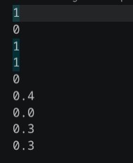
Figure 2.7: Example of values in in.data_{sta}

4. bridge file: in.connector

This file is used to define parameters mainly for forward modeling of receiver functions, as well as MCMC jump settings, multi-core processing, and post-run processing. All parameters can be modified in the script Setupdata/parameter.py using the following parameters:

MC_inversion_type: set to 1 for gradient style or 2 for B-spline style. Gradient style perturbs both velocity values and sublayer thickness values, while B-spline style uses quadratic B-splines to smooth the model. The B-spline style only provides variation in total group thickness; sublayer variations are smoothed and therefore not explicitly resolved.

RF_gaussian_width: input Gaussian factor used for forward modeling of receiver functions. This values need to consistent with gaussian factor that calculate the input receiver funtions.

MC_number_of_jump: number of jump to change the dimension on posterior distribution.

MC_number_of_iteration: defines how many samples are drawn at each jump.

MC_number_of_cores: defines how many cores use to run.

MC_percentage_post_process_select: defines the percentage of posterior models used to obtain the final model.

Depth_step: grid step for final model (in km).

modout_plot_type: define the plot style as layer-cake (0) or gradient (1).

MC_QC_thres: use the model quality control (1) or not (0). The quality control value set at the last row of file {Project}/data/{sta}data/in.connector the function name “goodmodel” on {Project}/Codes/MCMC_flex/CALmodel.C

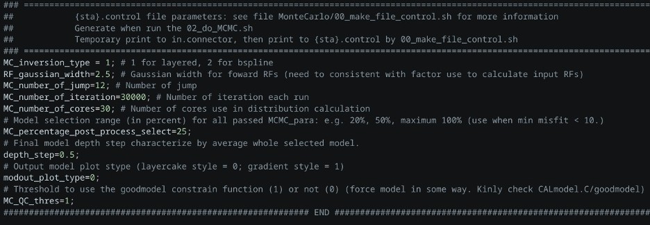
Figure 2.8: Location of parameters in SetupData/parameter.py that are transferred into the {Project}/data/{sta}_data/in.connector file for controlling the workflow.

⇒ After running the script 01_prepare_data.sh, the model for each station will be generated in {project}/data/{sta}_data/in.connector with the proper value structure.

The parameter values are arranged following the logic below:

Rows Information:

Row 1: MC_inversion_type.

Row 2: RF_gaussian_width.

Row 3: MC_number_of_jump.

Row 4: MC_number_of_iteration.

Row 5: MC_number_of_cores.

Row 6: MC_percentage_post_process_select.

Row 7: Depth_step.

Row 8: modout_plot_type.

Row 9: MC_QC_thres.

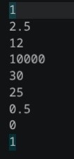
Figure 2.9: Example of {Project}/data/{sta}_data/in.connector file for controlling the workflow.