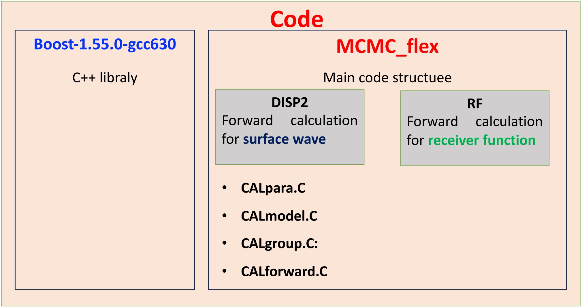
03. Importan functions

This part highlights several key functions in the workflow that you should consider in order to understand the overall process and reduce the time needed to get familiar with the code, especially if you want to improve the performance or apply new ideas. These functions are not touch to the core of Bayesian generator; instead, they handle communication between modules, model setup, posterior sampling, model quality control, posterior selection, and plotting styles to support result interpretation.

1. Switching between gradient to pure layercake: CALgroup.C/updategroup

This function is used to update the model used in the inversion process, which is internally represented in layer-cake style (parameterized as stacked layers with thickness and velocity). It controls the transformation from different input 1D model types (e.g., B-spline, layer-cake, gradient) into the layer-cake representation:

1. Updategroup1: convert from layer-cake like model to layer-cake–like model

2. Updategroup2: convert from B-spline like model to layer-cake–like model

3. Updategroup3: convert from gradient like model to layer-cake–like model

4. Updategroup4: convert from water layer model to layer-cake–like model (I am not sure what is this, but it may be used to handle the model where a water layer exists on top of the structure.)

Current setup for input layer-cake model and MCMC process, the function Updategroup1 calculate the velocity as linear interpolation velocity between two control points:

$$ V(z)=V_i+\frac{V_{i+1}-V_i}{Z_{i+1}-Z_i}(Z-Z_i)\tag{3.1} $$

Where:

• V(z) : velocity at depth z

• V_i and V_i+1: velocity at control depth i and i+1 with z located between them)

• z : depth between layers.

So it is become gradient style model. If you want to change back to layer-cake style, commend like for gradient style and uncommend the like for pure layer-cake. Then the V(z) is simply as”

$$ V(z) = V_{i} \tag{3.2} $$

or

$$ V(z) = \frac{\left( V_{i} + V_{i + 1} \right)}{2} \tag{3.3} $$

The V(z) calculation in updategroup1 that coresponding to equations (1.1) to (1.3) is listed here

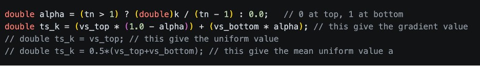
Figure 3.1: Location of Vs estimation when transferring from layer-cake input model in updategroup1.

2. How the misfit of the model is computed: CALmodel.C/compute_misfit

The misfit function measures the difference between the observed data and the synthetic data predicted from the current model. For each data point, the residual is first normalized by the data uncertainty:

a. The residual of data point ith is calculate as:

$$ r_{i} = \frac{\left( d_{obs,i} - d_{syn,i} \right)}{\sigma_{i}} \tag{3.4} $$

where:

• d_obs : observed data

• d_syn : synthetic data from the model

• \(\sigma_i\): uncertainty of the i-th data point

b. The misfit of each dataset then calculate as:

$$ {misfit}_{data} = \sqrt{\frac{1}{N}\sum_{i = 1}^{N}\left( r_{i} \right)^{2}} \tag{3.5} $$

This means the misfit is essentially the root-mean-square normalized residual. The normalization by the number of data points is important because it prevents datasets with more points from automatically giving a larger misfit just because they contain more samples.

c. After the individual misfit are computed, they are combined into a total misfit using weighting factors:

$$ m_{total} = w_{ph}m_{ph} + w_{gv}m_{gv} + w_{hv}m_{hv} + w_{rf}m_{rf} \tag{3.6} $$

where \(w_{ph}, w_{gv}, w_{hv}, w_{rf}\) denote the weights assigned to each dataset.

If equal weighting is chosen, the code distributes the weights equally among all available data types. If manual weighting is used, the user defines the weight for each data type, and the total should sum to 1.

d. Likelihood function: The likelihood function converts the misfit into a probability-like value used in the MCMC sampling. In general, the likelihood decreases as the misfit increases. A common form is:

$$ L = \exp\left( - \frac{1}{2}S \right) = \exp\left( - \frac{1}{2}\sum_{i = 1}^{N}\left( r_{i} \right)^{2} \right) \tag{3.7} $$

Then the likelihook for all the dataset express as:

$$ L = exp\left( - \frac{1}{2}\left\lbrack w_{ph}S_{ph} + w_{gv}S_{gv} + w_{hv}S_{hv} + w_{rf}S_{rf} \right\rbrack \right) \tag{3.8} $$

This means:

• smaller misfit \(\rightarrow\) larger likelihood

• larger misfit \(\rightarrow\) smaller likelihood

So models that fit the data better are more likely to be accepted during the MCMC process.

3. Model quality control: CALmodel.C/goodmodel

This option is activated when the last row of {Project}/data/{sta}_data/in.connector is set to 1. This setting can be controlled by the parameter MC_QC_thres in SetupData/parameter.py. when it active, the function CALmodel.C/goodmodel is used to constrain the data quality and model behavior as follows:
1. Check valid forward data (Vph, Gv, HV, RF): If any forward result is abnormal, the model is rejected immediately.
2. Check monotonic increase of Vs in sediment: So if a deeper sediment sublayer has lower Vs than the shallower one, the model is rejected.
3. Check monotonic increase of Vs in crust: So if a deeper crustal sublayer has lower Vs than the shallower one, the model is rejected.
4. Check monotonic increase of Vs in mantle: So if a deeper mantle sublayer has lower Vs than the shallower one, the model is rejected.
5. Check positive jump at sediment–crust boundary: The code checks the interface between sediment and crust. It requires the bottom sediment velocity to be smaller than the top crust velocity. If bottom sediment is greater than top crust, the model is rejected.
6. Check positive jump at crust–mantle boundary: The code also checks the interface between crust and mantle. It requires the bottom crust velocity to be smaller than the first mantle velocity. If bottom crust is greater than the mantle top, the model is rejected.
7. Check monotonic increase in sediment layers (use for MCMC in bspline style only): If sediment exists, the code checks that sediment Vs also increases with depth.
8. Check consistent ordering of spline/control points (use for MCMC in bspline style only): There is a QC check for spline-style models: (1) the second crust spline should not be smaller than the first. (2) the second mantle spline should not be smaller than the first. So the code is also checking that the top part of the spline model has a positive or non-negative trend.
9. Check positive velocity gradient at top of selected layers (use for MCMC in bspline style only): The code uses the vector vgrad to apply an additional positive-gradient check for selected groups. This means, for the groups listed in vgrad, the first two velocity values must satisfy.

Note: For each study, you need to turn these options on/off by commenting or uncommenting their corresponding code blocks.